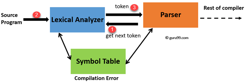
System Software and Compiler Design

Memory: ⦿ Memory consists of 8-bit bytes; any 3 consecutive bytes form a word (24 bits). All addresses on SIC are byte addresses ⦿ Words are addressed by the location of their lowest numbered byte. ⦿ There are total of 32,768 (215) bytes in the computer memory. Registers: There are five registers, all of which have special uses. Each register is 24 bits in length. Their mnemonics, numbers and uses are given in the following table.

Mnemonic	Number	Special Use
A	0	Accumulator; used for arithmetic operations
X	1	Index register; used for addressing
L	2	Linkage register; JSUB instruction stores the return address in this register
PC	8	Program counter; contains the address of the next instruction to be fetched for execution.
SW	9	Status word; contains a variety of information, including a Condition Code (CC)

Data Formats: ⦿Integers are stored as 24-bit binary numbers. ⦿2’s complement representation is used for negative values. ⦿characters are stored using their 8-bit ASCII codes. ⦿There is no floating-point hardware on the standard version of SIC. Instruction Formats: All machine instructions on the standard version of SIC have the 24-bit format:

8	       1	           15
opcode	       x	           Address

Addressing Modes: There are two addressing modes available, indicated by the setting of the x bit in the instruction.

Mode	Indication	Target Address Calculation
Direct	x=0	TA= address
Indexed	x=1	TA= address + (X)

Parentheses are used to indicate the contents of a register or a memory location. For example, (X) represents the contents of register X. Direct Addressing Mode:

 Example: LDA     TEN		LDA – 00
 opcode	  x	                                 TEN
 0 0 0 0   0 0 0 0	  0	        0 0 1    0 0 0 0    0 0 0 0    0 0 0 0
 Effective Address (EA) = 1000
 Content of the address 1000 is loaded to Accumulator.
 
 

Indexed Addressing Mode: Example: STCH BUFFER, X

 
 opcode	  x	                          BUFFER
 0 0 0 0   0 1 0 0	  1	        0 0 1    0 0 0 0    0 0 0 0    0 0 0 0

Effective Address (EA) = 1000 + [X] = 1000 + content of the index register X The Accumulator content, the character is loaded to the Effective address. Instruction Set: SIC provides, load and store instructions (LDA, LDX, STA, STX, etc.). Integer arithmetic operations: (ADD, SUB, MUL, DIV, etc.). All arithmetic operations involve register A and a word in memory, with the result being left in the register. Two instructions are provided for subroutine linkage. COMP compares the value in register A with a word in memory, this instruction sets a condition code CC to indicate the result. There are conditional jump instructions: (JLT, JEQ, JGT), these instructions test the setting of CC and jump accordingly. JSUB jumps to the subroutine placing the return address in register L, RSUB returns by jumping to the address contained in register L. Input and Output: Input and Output are performed by transferring 1 byte at a time to or from the rightmost 8 bits of register A (accumulator). The Test Device (TD) instruction tests whether the addressed device is ready to send or receive a byte of data. Read Data (RD), Write Data (WD) are used for reading or writing the data.

Machine-Dependent Assembler Features: ➜Instruction formats and addressing modes ➜Program relocation. Instruction formats and Addressing Modes The instruction formats depend on the memory organization and the size of the memory. In SIC machine the memory is byte addressable. Word size is 3 bytes. So the size of the memory is 2^12 bytes. Accordingly it supports only one instruction format. It has only two registers: register A and Index register. Therefore the addressing modes supported by this architecture are direct, indirect, and indexed. Whereas the memory of a SIC/XE machine is. 220 bytes (1 MB). This supports four different types of instruction types, they are:   1 byte instruction   2 byte instruction   3 byte instruction   4 byte instruction Instructions can be: –-- Instructions involving register to register –-- Instructions with one operand in memory, the other in Accumulator (Single operand instruction) --– Extended instruction format Addressing Modes are: –-- Index Addressing(SIC): Opcode m, x –-- Indirect Addressing: Opcode @m –-- PC-relative: Opcode m --– Base relative: Opcode m –-- Immediate addressing: Opcode #c Translations for the Instruction involving Register-Register addressing mode: During pass 1 the registers can be entered as part of the symbol table itself. The value for these registers is their equivalent numeric codes. During pass2, these values are assembled along with the mnemonics object code. If required a separate table can be created with the register names and their equivalent numeric values. Translation involving Register-Memory instructions: In SIC/XE machine there are four instruction formats and five addressing modes. For formats and addressing modes. Among the instruction formats, format -3 and format-4 instructions are Register-Memory type of instruction. Program relocation ➜The actual starting address of the program is not known until load time ➜An object program that contains the information necessary to perform this kind of modification is called a relocatable program ➜No modification is needed: operand is using program-counter relative or base relative addressing ➜The only parts of the program that require modification at load time are those that specified direct (as opposed to relative) addresses ➜Modification record  ⦿Col. 2-7 Starting location of the address field to be modified, relative to the beginning of the program (Hex) ➜Col. 8-9 Length of the address field to be modified, in half-bytes (Hex) Machine independent assembler feature: Literals Symbol-defining statements Expressions Program block Control sections and program linking Literals  ➤ Write the value of a constant operand as a part of the instruction that uses it Such an operand is called a literal  ➤ Avoid having to define the constant elsewhere in the program and make up a label for it  ➤ A literal is identified with the prefix =, which is followed by a specification of the literal value  ➤ Examples of literals in the statements:

o45	001A	ENDFIL	LDA	=C’EOF’    032010
o215	1062	WLOOP	TD	=X’05’	   E32011 

 ➤ With a literal, the assembler generates the specified value as a constant at some other memory location  ➤ The address of this generated constant is used as the target address for the machine instruction  ➤ All of the literal operands used in the program are gathered together into one or more literal pools  ➤ Normally literals are placed into a pool at the end of the program  ➤ A LTORG statement creates a literal pool that contains all of the literal operands used since the previous LTORG  ➤ Most assembler recognize duplicate literals: the same literal used in more than one place and store only one copy of the specified data value  ➤ LITTAB (literal table): contains the literal name, the operand value and length, and the address assigned to the operand when it is placed in a literal pool Expressions  Assembler allow arithmetic expressions formed according to the normal rules using the operator +, -, *, and /  Individual terms in the expression may be constants, user-defined symbols, or special terms  The most common such special term is the current value of the location counter (designed by *)  Expressions are classified as either absolute expressions or relative expressions Program Block  Program blocks: segments of code that are rearranged within a single object unit  Control sections: segments that are translated into independent object program units  USE indicates which portions of the source program belong to the various blocks Control section  References between control sections are called external references  The assembler generates information for each external reference that will allow the loader to perform the required linking  The EXTDEF (external definition) statement in a control section names symbol, called external symbols, that are define in this section and may be used by other sections  The EXTREF (external reference) statement names symbols that are used in this control section and are defined elsewhere Define record (D) ⦿  Col. 2-7 Name of external symbol defined in this control section ⦿  Col. 8-13 Relative address of symbol within this control section (Hex) ⦿  Col. 14-73 Repeat information in Col. 2-13 for other external symbols Refer record (R) ⦿  Col. 2-7 Name of external symbol referred to in this control section ⦿  Col. 8-73 Names of other external reference symbols Modification record (revised : M) ⦿  Col. 2-7 Starting address of the field to be modified, relative to the beginning of the control section (Hex) ⦿  Col. 8-9 Length of the field to be modified, in half-bytes (Hex) ⦿  Col. 10 Modification flag (+ or -) ⦿  Col. 11-16 External symbol whose value is to be added to or subtracted from the indicated field

Program relocation

Ø The actual starting address of the program is not known until load time

Ø An object program that contains the information necessary to perform this kind of modification is called a relocatable program

Ø No modification is needed: operand is using program-counter relative or base relative addressing

Ø The only parts of the program that require modification at load time are those that specified direct (as opposed to relative) addresses

Ø Modification record

        o Col. 2-7 Starting location of the address field to be modified, relative to the           beginning of the program (Hex)

Col. 8-9  Length of the address field to be modified, in half-bytes (Hex)

Sometimes it is required to load and run several programs at the same time. The system must be able to load these programs wherever there is place in the memory. Therefore the exact starting is not known until the load time.

Absolute Program

In this the address is mentioned during assembling itself. This is called Absolute Assembly.

 

Consider the instruction:

55101B  LDA   THREE    00102D

· This statement says that the register A is loaded with the value stored at location 102D. Suppose it is decided to load and execute the program at location 2000 instead of location 1000.

· Then at address 102D the required value which needs to be loaded in the register A is no more available. The address also gets changed relative to the displacement

of the program. Hence we need to make some changes in the address portion of the instruction so that we can load and execute the program at location 2000.

 

· Apart from the instruction which will undergo a change in their operand address value as the program load address changes. There exist some parts in the program which will remain same regardless of where the program is being loaded.

 

· Since assembler will not know actual location where the program will get loaded, it cannot make the necessary changes in the addresses used in the program. However, the assembler identifies for the loader those parts of the program which need modification.

 

· An object program that has the information necessary to perform this kind of modification is called the relocatable program.

 The Algorithm for Pass 1:

The Algorithm for Pass 2:

The operation of absolute loader is very simple. The object code is loaded to specified locations in the memory. At the end the loader jumps to the specified address to begin execution of the loaded program. The role of absolute loader is as shown in the figure 4.4.

The advantage of absolute loader is simple and efficient. But the disadvantages are, the need for programmer to specify the actual address, and, difficult to use subroutine libraries.

The algorithm for this type of loader is given here. The object program and, the object program loaded into memory by the absolute loader are also shown. Each byte of assembled code is given using its hexadecimal representation in character form. Easy to read by human beings. Each byte of object code is stored as a single byte. Most machine store object programs in a binary form, and we must be sure that our file and device conventions do not cause some of the program bytes to be interpreted as control characters.

Begin

read Header record

verify program name and length

read first Text record

while record type is <> ‘E’ do

begin

{if object code is in character form, convert into internal representation} move object code to specified location in memory read next object program record

end

jump to address specified in End record

end

Pass 1:

Begin

get PROOADDR from operating system

set CSADDR to PROOADDR {for first control section}

while not end of input do

begin

read next input record {Header record for control section}

set CSLTH to control section length

search ESTAB for control section name

if found then

set error flag {duplicate external symbol}

else

enter control section name into ESTAB with value CSADDR

while record type ~ 'E' do

begin

read next input record

if record type = 'D' then

for each symbol in the record do

begin

search ESTAB for symbol name

if found then

set error flag (duplicate external symbol)

else

enter symbol into ESTAB with value(CSADDR + indicated address)

end {for}

end {while ~ 'E'}

add CSLTH to CSADDR {starting address for next control section}

end {while not EOF}

end {Pass 1}

The scheme that postpones the linking functions until execution. A subroutine is loaded and linked to the rest of the program when it is first called – usually called dynamic linking, dynamic loading or load on call. The advantages of dynamic linking are, it allow several executing programs to share one copy of a subroutine or library. In an object oriented system, dynamic linking makes it possible for one object to be shared by several programs. Dynamic linking provides the ability to load the routines only when (and if) they are needed. The actual loading and linking can be accomplished using operating system service request.

 1) Lexical Analyzer

— The first phase of compiler is lexical analyzer it reads stream of characters in the source program

— Groups the characters into meaningful sequences – lexemes

— For each lexeme, a token is produced as output

—  <token-name , attribute-value>

Token-name : symbol used during syntax analysis

Attribute-value : an entry in the symbol table for this token

— Information from symbol table is needed for syntax analysis and code generation

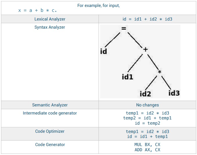
— Consider the following assignment statement 

2) Syntax Analysis

The second phase of compiler is  syntax analysis  is also  called Parsing

— Parser uses the tokens to create a tree-like intermediate representation

— Depicts the grammatical structure of the token stream

— Syntax tree is one such representation

                                 Interior node – operation

                                 Children  - arguments of the operation

Other phases use this syntax tree to help analyze source program and generate target program

3) Semantic Analysis

The third phase of compiler is Semantic Analyzer

— Checks semantic consistency with language using:

                               Syntax tree  and Information in symbol table

— Gathers type information and save in syntax tree or symbol table

— Type Checks each operator for matching operands

                               Ex: Report error if floating point number is used as index of an array

— Coercions or type conversions

                         Binary arithmetic operator applied to a pair of integers or floating point numbers

                           If applied to floating point and integer, compiler may convert integer to floating-

                            point number

4) Intermediate Code Generation

     After syntax and semantic analysis  Intermediate Code Generation is the fourth  phase of compiler

— Compilers generate machine-like intermediate representation

— This intermediate representation should have the two properties:

                         Should be easy to produce

                         Should be easy to translate into target machine

             Three-address code

— Sequence of assembly-like instructions with three operands per instruction

— Each operand acts like a register

                        Points to be noted about three-address instructions are:

— Each assignment instruction has at most one operator on the right side

— Compiler must generate a temporary name to hold the value computed by a three-address instruction

— Some instructions have fewer than three operands

 

5) Code Optimization

            Attempt to improve the target code

— Faster code, shorter code or target code that consumes less power

                        Optimizer can deduce that

— Conversion of 60 from int to float can be done once  at compile time

— So, the inttofloat can be eliminated by replacing 60 with 60.0

— t3 is used only once to transmit its value to id1

6) Code Generation

— Takes intermediate representation as input

— Maps it into target language

— If target language is machine code

                        Registers or memory locations are selected for each of the variables used

                        Intermediate instructions are translated into sequences of machine instructions

                        performing the same task

— Assignment of registers to hold variables is a crucial aspect

The compilation process is a sequence of various phases. Each phase takes input from its previous stage, has its own representation of source program, and feeds its output to the next phase of the compiler. Let us understand the phases of a compiler.

---

Lexical Analysis The first phase of scanner works as a text scanner. This phase scans the source code as a stream of characters and converts it into meaningful lexemes. Lexical analyzer represents these lexemes in the form of tokens as:

<token-name, attribute-value> 

---

Syntax Analysis The next phase is called the syntax analysis or parsing. It takes the token produced by lexical analysis as input and generates a parse tree (or syntax tree). In this phase, token arrangements are checked against the source code grammar, i.e. the parser checks if the expression made by the tokens is syntactically correct.

---

Semantic Analysis Semantic analysis checks whether the parse tree constructed follows the rules of language. For example, assignment of values is between compatible data types, and adding string to an integer. Also, the semantic analyzer keeps track of identifiers, their types and expressions; whether identifiers are declared before use or not etc. The semantic analyzer produces an annotated syntax tree as an output.

---

Intermediate Code Generation After semantic analysis the compiler generates an intermediate code of the source code for the target machine. It represents a program for some abstract machine. It is in between the high-level language and the machine language. This intermediate code should be generated in such a way that it makes it easier to be translated into the target machine code.

---

Code Optimization The next phase does code optimization of the intermediate code. Optimization can be assumed as something that removes unnecessary code lines, and arranges the sequence of statements in order to speed up the program execution without wasting resources (CPU, memory).

---

Code Generation In this phase, the code generator takes the optimized representation of the intermediate code and maps it to the target machine language. The code generator translates the intermediate code into a sequence of (generally) re-locatable machine code. Sequence of instructions of machine code performs the task as the intermediate code would do.

---

Symbol Table It is a data-structure maintained throughout all the phases of a compiler. All the identifier's names along with their types are stored here. The symbol table makes it easier for the compiler to quickly search the identifier record and retrieve it. The symbol table is also used for scope management.

LEXICAL ANALYSIS is the very first phase in the compiler designing. A Lexer takes the modified source code which is written in the form of sentences . In other words, it helps you to convert a sequence of characters into a sequence of tokens. The lexical analyzer breaks this syntax into a series of tokens. It removes any extra space or comment written in the source code. Programs that perform lexical analysis are called lexical analyzers or lexers. A lexer contains tokenizer or scanner. If the lexical analyzer detects that the token is invalid, it generates an error. It reads character streams from the source code, checks for legal tokens, and pass the data to the syntax analyzer when it demands.

---

Example

How Pleasant Is The Weather?

See this example; Here, we can easily recognize that there are five words How Pleasant, The, Weather, Is. This is very natural for us as we can recognize the separators, blanks, and the punctuation symbol.

---

 HowPl easantIs Th ewe ather?

Now, check this example, we can also read this. However, it will take some time because separators are put in the Odd Places. It is not something which comes to you immediately.

The main task of lexical analysis is to read input characters in the code and produce tokens. Lexical analyzer scans the entire source code of the program. It identifies each token one by one. Scanners are usually implemented to produce tokens only when requested by a parser. Here is how this works-

1. "Get next token" is a command which is sent from the parser to the lexical analyzer.
2. On receiving this command, the lexical analyzer scans the input until it finds the next token.
3. It returns the token to Parser.

Lexical Analyzer skips whitespaces and comments while creating these tokens. If any error is present, then Lexical analyzer will correlate that error with the source file and line number.

---

Lexical analyzer performs below given tasks:

• Helps to identify token into the symbol table
• Removes white spaces and comments from the source program
• Correlates error messages with the source program
• Helps you to expands the macros if it is found in the source program
• Read input characters from the source program

Example of Lexical Analysis, Tokens, Non-Tokens Consider the following code that is fed to Lexical Analyzer

#include <stdio.h>
    int maximum(int x, int y) {
        // This will compare 2 numbers
        if (x > y)
            return x;
        else {
            return y;
        }
    }

---

Examples of Tokens created

 

Lexeme	Token
int	Keyword
maximum	Identifier
(	Operator
int	Keyword
x	Identifier
,	Operator
int	Keyword
Y	Identifier
)	Operator
{	Operator
If	Keyword

---

 

Examples of Nontokens

Type	Examples
Comment	// This will compare 2 numbers
Pre-processor directive	#include <stdio.h>
Pre-processor directive	#define NUMS 8,9
Macro	NUMS
Whitespace	/n /b /t

The lexical analyzer scans the input from left to right one character at a time. It uses two pointers begin ptr(bp) and forward to keep track of the pointer of the input scanned.

---

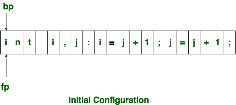
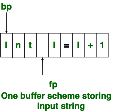
Initially both the pointers point to the first character of the input string as shown below The forward ptr moves ahead to search for end of lexeme. As soon as the blank space is encountered, it indicates end of lexeme. In above example as soon as ptr (fp) encounters a blank space the lexeme “int” is identified. The fp will be moved ahead at white space, when fp encounters white space, it ignore and moves ahead. then both the begin ptr(bp) and forward ptr(fp) are set at next token. 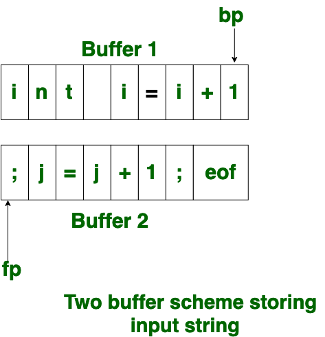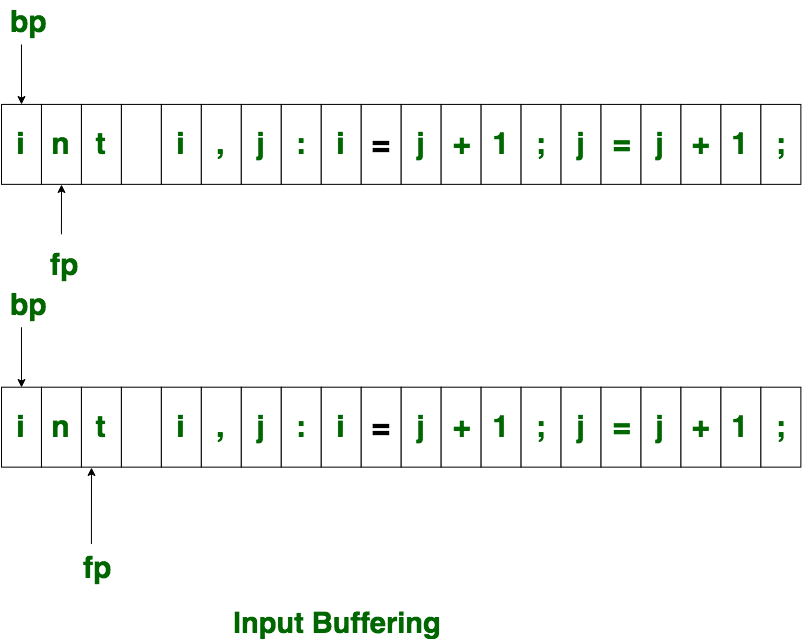The input character is thus read from secondary storage, but reading in this way from secondary storage is costly. hence buffering technique is used.A block of data is first read into a buffer, and then second by lexical analyzer. there are two methods used in this context: One Buffer Scheme, and Two Buffer Scheme. These are explained as following below.

---

• One Buffer Scheme: In this scheme, only one buffer is used to store the input string but the problem with this scheme is that if lexeme is very long then it crosses the buffer boundary, to scan rest of the lexeme the buffer has to be refilled, that makes overwriting the first of lexeme.
• Two Buffer Scheme: To overcome the problem of one buffer scheme, in this method two buffers are used to store the input string. the first buffer and second buffer are scanned alternately. when end of current buffer is reached the other buffer is filled. the only problem with this method is that if length of the lexeme is longer than length of the buffer then scanning input cannot be scanned completely. Initially both the bp and fp are pointing to the first character of first buffer. Then the fp moves towards right in search of end of lexeme. as soon as blank character is recognized, the string between bp and fp is identified as corresponding token. to identify, the boundary of first buffer end of buffer character should be placed at the end first buffer. Similarly end of second buffer is also recognized by the end of buffer mark present at the end of second buffer. when fp encounters first eof, then one can recognize end of first buffer and hence filling up second buffer is started. in the same way when second eof is obtained then it indicates of second buffer. alternatively both the buffers can be filled up until end of the input program and stream of tokens is identified. This eof character introduced at the end is calling Sentinel which is used to identify the end of buffer.

The figure below shows the processing of an object program using Linkage editor. A linkage editor produces a linked version of the program – often called a load module or an executable image – which is written to a file or library for later execution. The linked program produced is generally in a form that is suitable for processing by a relocating loader. Some useful functions of Linkage editor are, an absolute object program can be created, if starting address is already known. New versions of the library can be included without changing the source program. Linkage editors can also be used to build packages of subroutines or other control sections that are generally used together. Linkage editors often allow the user to specify that external references are not to be resolved by automatic library search – linking will be done later by linking loader – linkage editor + linking loader – savings in space

The Goal of program linking is to resolve the problems with external references (EXTREF) and external definitions (EXTDEF) from different control sections. EXTDEF (external definition) - The EXTDEF statement in a control section names symbols, called external symbols, that are defined in this (present) control section and may be used by other sections.

---

ex: EXTDEF BUFFER, BUFFEND, LENGTH EXTDEF LISTA, ENDA EXTREF (external reference) - The EXTREF statement names symbols used in this (present) control section and are defined elsewhere. ex: EXTREF RDREC, WRREC EXTREF LISTB, ENDB, LISTC, ENDC

---

How to implement EXTDEF and EXTREF The assembler must include information in the object program that will cause the loader to insert proper values where they are required – in the form of Define record (D) and, Refer record(R). Define record The format of the Define record (D) along with examples is as shown here. Col. 1 D Col. 2-7 Name of external symbol defined in this control section Col. 8-13 Relative address within this control section (hexadecimal) Col.14-73 Repeat information in Col. 2-13 for other external symbols

➜ It supports a wide variety of macro facilities and structured programming idioms, including high-level constructions for looping, procedure calls and alternation (therefore, MASM is an example of a high-level assembler). ➜ MASM is one of the few Microsoft development tools for which there was no separate 16-bit and 32-bit version. ➜ Assembler affords the programmer looking for additional performance a three pronged approach to performance based solutions. ➜ MASM can build very small high performance executable files that are well suited where size and speed matter. ➜ When additional performance is required for other languages, MASM can enhance the performance of these languages with small fast and powerful dynamic link libraries. ➜ For programmers who work in Microsoft Visual C/C++, MASM builds modules and libraries that are in the same format so the C/C++ programmer can build modules or libraries in MASM and directly link them into their own C/C++ programs. This allows the C/C++ programmer to target critical areas of their code in a very efficient and convenient manner, graphics manipulation, games, very high speed data manipulation and processing, parsing at speeds that most programmers have never seen, encryption, compression and any other form of information processing that is processor intensive. ➜ MASM32 has been designed to be familiar to programmers who have already written API based code in Windows. The invoke syntax of MASM allows functions to be called in much the same way as they are called in a high level compiler.

---

The linkage editor is a processing program that accepts object modules, load modules, control statements, and options as input. It combines these modules, according to the requirements defined by the control statements and options, into a single output load module that can be stored in a partitioned data set program library and loaded into storage for execution by the program management loader. The linkage editor also provides other processing and service facilities, including creating overlay programs, aiding program modification, and building and editing system libraries. It supports addressing and residence mode attributes in both 24- and 31-bit addressing ranges. It does not support program objects or the (GOFF) object format. All of the services of the linkage editor can be performed by the binder.

Machine-Dependent Loader Features

Absolute loader is simple and efficient, but the scheme has potential disadvantages One of the most disadvantage is the programmer has to specify the actual starting address, from where the program to be loaded. This does not create difficulty, if one program to run, but not for several programs. Further it is difficult to use subroutine libraries efficiently.

This needs the design and implementation of a more complex loader. The loader must provide program relocation and linking, as well as simple loading functions.

 

Relocation

The concept of program relocation is, the execution of the object program using any part of the available and sufficient memory. The object program is loaded into memory wherever there is room for it. The actual starting address of the object program is not known until load time. Relocation provides the efficient sharing of the machine with larger memory and when several independent programs are to be run together. It also supports the use of subroutine libraries efficiently. Loaders that allow for program relocation are called relocating loaders or relative loaders.

Methods for specifying relocation

Use of modification record and, use of relocation bit, are the methods available for specifying relocation. In the case of modification record, a modification record M is used in the object program to specify any relocation. In the case of use of relocation bit, each instruction is associated with one relocation bit and, these relocation bits in a Text record is gathered into bit masks.

Modification records are used in complex machines and is also called Relocation and Linkage Directory (RLD) specification. The format of the modification record (M) is as follows. The object program with relocation by Modification records is also shown here.

Modification record

col 1:	M
col 2-7:	relocation address
col 8-9:	length (halfbyte)
col 10:	flag (+/-)
col 11-17:	segment name

 

HΛCOPY Λ000000 001077

TΛ000000 Λ1DΛ17202DΛ69202DΛ48101036Λ…Λ4B105DΛ3F2FECΛ032010

TΛ00001DΛ13Λ0F2016Λ010003Λ0F200DΛ4B10105DΛ3E2003Λ454F46

TΛ001035 Λ1DΛB410ΛB400ΛB440Λ75101000Λ…Λ332008Λ57C003ΛB850

TΛ001053Λ1DΛ3B2FEAΛ134000Λ4F0000ΛF1Λ..Λ53C003ΛDF2008ΛB850

TΛ00070Λ07Λ3B2FEFΛ4F0000Λ05

MΛ000007Λ05+COPY

MΛ000014Λ05+COPY

MΛ000027Λ05+COPY

EΛ000000

The relocation bit method is used for simple machines. Relocation bit is 0: no modification is necessary, and is 1: modification is needed. This is specified in the columns 10-12 of text record (T), the format of text record, along with relocation bits is as follows.

Text record

col 1: T

col 2-7: starting address

col 8-9: length (byte)

col 10-12: relocation bits

col 13-72: object code

Twelve-bit mask is used in each Text record (col:10-12 – relocation bits), since each text record contains less than 12 words, unused words are set to 0, and, any value that is to be

modified during relocation must coincide with one of these 3-byte segments. For absolute loader, there are no relocation bits column 10-69 contains object code. The object program with relocation by bit mask is as shown below. Observe FFC - means all ten words are to be modified and, E00 - means first three records are to be modified.

H_ΛCOPY _Λ000000 00107A

T_Λ000000_Λ1E_ΛFFC_Λ140033_Λ481039_Λ000036_Λ280030_Λ300015_Λ…_Λ3C0003 _Λ …

T_Λ00001E_Λ15_ΛE00_Λ0C0036_Λ481061_Λ080033_Λ4C0000_Λ…_Λ000003_Λ000000

T_Λ001039_Λ1E_ΛFFC_Λ040030_Λ000030_Λ…_Λ30103F_ΛD8105D_Λ280030_Λ...

T_Λ001057_Λ0A_Λ800_Λ100036_Λ4C0000_ΛF1_Λ001000

T_Λ001061_Λ19_ΛFE0_Λ040030_ΛE01079_Λ…_Λ508039_ΛDC1079_Λ2C0036_Λ...

E_Λ000000

 Program Linking

The Goal of program linking is to resolve the problems with external references (EXTREF) and external definitions (EXTDEF) from different control sections.

EXTDEF (external definition) - The EXTDEF statement in a control section names symbols, called external symbols, that are defined in this (present) control section and may be used by other sections.

ex: EXTDEF BUFFER, BUFFEND, LENGTH

EXTDEF LISTA, ENDA

EXTREF (external reference) - The EXTREF statement names symbols used in this (present) control section and are defined elsewhere.

ex: EXTREF RDREC, WRREC EXTREF LISTB, ENDB, LISTC, ENDC

 

 

The compilation process is a sequence of various phases. Each phase takes input from the previous, and passes the output on to the next phase.

LEXICAL ANALYSIS

The first phase of compiler works as a text scanner. The lexical analyzer scans the source code as a stream of characters and converts it into meaningful lexemes of the form .

SYNTAX ANALYSIS

It takes the token produced by lexical analysis as input and generates a parse tree (or syntax tree). Token arrangements are checked against the source code grammar.

SEMANTIC ANALYSIS

Checks whether the parse tree constructed follows the rules of language. E.g. assignment of values is between compatible data types, and adding string to an integer. It keeps track of identifiers, their types and expressions. It produces an annotated syntax tree as an output.

INTERMEDIATE CODE GENERATION

After semantic analysis the compiler generates an intermediate code of the source code for the target machine. It represents a program for some abstract machine. It is generated in such a way that it makes it easier to be translated into the target machine code.

CODE OPTIMIZATION

Optimization can be assumed as something that removes unnecessary code lines, and arranges the sequence of statements in order to speed up the program execution without wasting resources. CODE GENERATION This phase takes the optimized representation of the intermediate code and maps it to the target machine language (sequence of re-locatable machine code).

 

A compiler scans the entire program and translates it as a whole into relocatable machine code. It takes large amount of time to analyze the source code but the overall execution time is comparatively faster. It generates intermediate object code which further requires linking, hence requires more memory. It generates the error message only after scanning the whole program. An interpreter translates program one statement at a time. It takes less amount of time to analyze the source code but the overall execution time is slower. No intermediate object code is generated, hence are memory efficient. It continues translating the program until the first error is met, in which case it stops.

A language processing system consists of 4 main units; the preprocessor, the compiler, the assembler, and the linker/loader. The preprocessor collects the source program split into modules and files, expands macros into language statement. The compiler takes modified source program and generates machine language code. The assembler takes the machine language code and converts it into relocatable object code. The linker links pieces of large programs that need to be compiled in pieces. It also resolves external memory references. The loader loads all the executables into memory.

 

We often have to look one or more characters beyond the next lexeme, before we can be sure that we have the right lexeme.

For example, the symbols '<' or '=' could be the beginning of '<<', '<=', ==', etc.

Hence we need two buffer schemes to handle the large lookahead safely. The buffer pairs consist of a lexeme begin pointer (lbp) and a forward pointer (fp).

The lexeme begin pointer marks the beginning of the current lexeme, and the forward pointer scans ahead until a pattern match is found.

This concept is called Input Buffering.

When using a single buffer scheme, if the end of the current file/block is reached before the expression ends, the lexical analyzer might return an unexpected token.

For example, for input string E = M * C ** 2

...	...	E	=	M	*	C	*	EOF	...	...
							lbp   ↑	fp  ↑

 

 

When EOF is reached in the middle of the expression, the lexical analyzer emits '*' as a token; reloads the input buffer, emits the next '*' as another token.

Two '*'s are returned instead of '**', hence invalidating the expression.

This drawback is overcome by using two buffer schemes.

...	E	=	M	*	C	*	EOF	...
						lbp ↑

 

...	*	2	EOF	...
		fp  ↑

When we use two buffers, when the input ends prematurely, the other buffer is loaded with the next file’s contents. Hence, the forward pointer moves to the next file to process the continuing input. The lexical analyzer hence emits '**' as the token.

Transition diagrams depict the actions that take place when a lexical analyzer is called by the parser to get the next token.

We can use a transition diagram to keep track of information about the characters that are seen as the forward pointer scans the input. We do so by moving position to position in the diagrams as the characters are read.

 

There are two ways, you can handle reserved words that look like identifiers:

► Put the reserved words in a symbol table initially, with a field indicating that they’re not ordinary identifiers, and tells what tokens do they represent.

When we find an identifier, a call to installID() places it in the symbol table if it’s not already there, and returns a pointer to the symbol table entry for the lexeme found. Any identifier not in the table is recognized as an 'id’.

► Create separate transition diagrams for each keyword, consisting of states representing the situation the keyword is to be detected.

The diagram consists of states representing each letter in the keyword, and check if the identifier has ended, with proper suffix detection. For e.g. 'then' should not be matched in 'thenextstep'.

A generated analyzer is a software tool that automatically constructs a lexical analyzer from a program in the lex language.

The lex compiler generates a transition table for a finite automaton from the regular expressions in the lex specification.

The lexical analyzer consists of finite automaton simulator that uses the transition table to look for the regular expression patterns in the input buffer.

► Reads characters in the source program and groups them into meaningful sequences called lexemes.

► Produces as output a token of the form <token_name, attribute_value> and passes it to the next phase syntax analysis.

► Token class - The symbol for this token to be used during syntax analysis.

► Attribute points to symbol table entry for this token.

► Role of lexical analyzer

-Remove comments & white spaces

-Macros expansion

-Read input characters from source program & group them into lexemes.

-Produce as output a source of tokens, interact with symbol table.

System Software -

• System software is machine dependent.
• System software focus is on the computing system.
• Its a general purpose software.
• System Software programming is complex than application software.
• Without system software, system can’t run.
• Examples: Operating system, compiler, assembler.

Application Software -

• Application software is not dependent on the underlying hardware.
• Application software provides solution to a problem.
• While its a specific purpose software.
• Application software programming is simpler as comparison to system software.
• While without application software system always runs.
• Examples: Antivirus, Microsoft office.